Ithaca High School Math Seminar Lesson 2-9

Date: 2023.11.30

Humanity has known about several fundamental mathematical results for hundreds of years, such as the fundamental theorem of calculus. Other results are significantly older, such as a the number of Platonic solids, which we've known about for thousands of years. Today we'll do something unusual in that we'll explore a topic less than 50 years old.

In the process we'll take advantage of the astonishing development of computer hardware over a similar timeframe to create images in microseconds that were impossible to compute 50 years ago. It's time to make some fractals, such as the image below.

Step 1: Iterate z ↦ z² + c for complex z and fixed c

Complex numbers can be thought of as pairs of real numbers satisfying an addition and multiplication rule. There are heaps of different ways of thinking about complex numbers (each of which provide different explanations for complex number phenomena), but thinking of them in terms of pairs will be enough for today.

When complex numbers are considered as pair of real numbers (a,b), they add in an intuitive way. For complex numbers (a,b) and (c,d), we define (a,b) + (c,d) = (a + c, b + d). Multiplication is more complicated. It is not defined as (a,b) × (c,d) = (ac, bd). Instead, we define (a,b) × (c,d) = (ac - bd, ad + bc).

From this perspective, the multiplication of complex numbers can appear weird, although it has a natural geometric interpretation in terms of lengths and angles. The length / norm / modulus |(a,b)| of a complex number is just its distance from the origin when considered as a point in the Euclidean plane. That is, |(a,b)| = √(a² + b²).

Since coordinates of pixels are pairs of real numbers, we can interpret them as complex numbers. Let's normalize pixel coordinates so that the vertical range of the screen is [-3,3], and plot all the complex numbers whose length is not greater than 2.

#version 330

uniform vec2 resolution;

void main(void) 
{
    vec2 pos = 3 * (2 * gl_FragCoord.xy - resolution) / resolution.y;
    
    vec4 color1  = vec4(1,1,1,1);
    vec4 color2  = vec4(0,0,0,1);
    
    bool in_R = length(pos) <= 2;
    
    gl_FragColor = float(in_R) * color1 + float(! in_R) * color2;
}

The result is a disk, just as we would expect. But what happens if we multiplied a complex number with itself several times, and then took the resulting length? What kind of shape do we then get when we plot the lengths that are less than 2?

This is easy to do in a fragment shader; we can simply replace the in_R line with the following code.

    vec2 zn = pos;
    zn = vec2(zn.x * zn.x - zn.y * zn.y, 2 * zn.x * zn.y);
    bool in_R = length(zn) <= 2;

Task: Derive the middle line in the code above from the definition of complex number multiplication.

The result is a slightly smaller disk. With the geometric interpretation of complex number multiplication, this is expected too. Taking higher powers results in slightly smaller disks, as we can see if we iterate the process. In lesson 2-2 we made extensive use of for loops to draw different regular polygons; we can likewise use for loops here to take higher powers. Calculating z⁸ is just ((z²)²)², which can easily calculate compute in by replacing the middle line above with the following code.

    for (int i = 0; i < 3; i += 1) {
        zn = vec2(zn.x * zn.x - zn.y * zn.y, 2 * zn.x * zn.y);
    }

The result is indeed a smaller disk.

Task: Create an even smaller disk by calculating z⁶⁴ for each pixel instead and then seeing if the resulting length is smaller than or equal to 2.

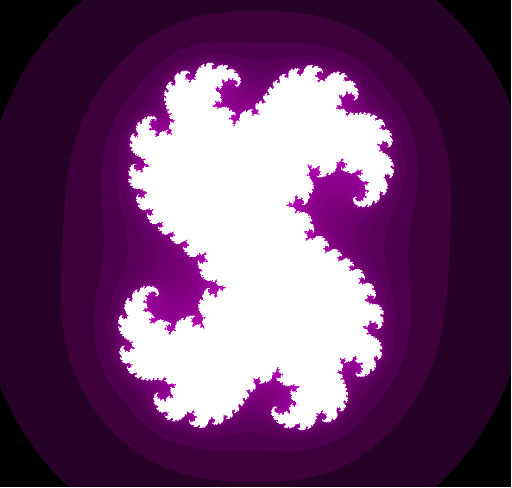
As is so often the case in mathematics, unexpected behavior, and sometimes beauty, can come about by slightly modifying something with regular behavior. What happens if in each iteration of the loop, we added a complex number before squaring?

Task: Modify the loop so that in each iteration zn² - (0.5,0.5) is calculated instead of zn².

The result is weird, but symmetrical, blob. What happens if we increase the number of loop iterations? We could do this by manually changing the iteration limit, but there is a more fun way of doing this.

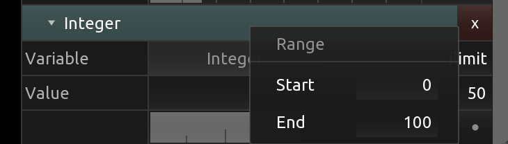
Let us add in a uniform which will control the number of loop iterations. In the right-side bar in KodeLife, if we create a new constant Integer parameter called ilimit (revisit lesson 2-5 if you would like a reminder of how to do this), set its range to be 0 and 100, we can then use this value in the code.

Underneath the resolution uniform we add the line

  uniform int ilimit;

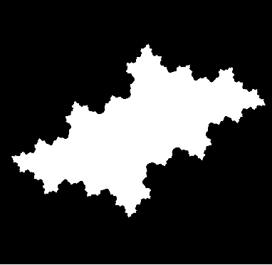
and then adjust the limit in the for loop to be ilimit. For example, when ilimit is set to 10, the region looks like the following.

Task: Add in a slider, increase ilimit past 10, and observe how the resulting fractal grows! You may want to adjust the vertical screen range from [-3,3] to [-1,1] to get better images.

Step 2: Add in mouse interactivity

We chose the constant c in the z ↦ z² loop body to be (-0.5,-0.5)... but what happens with other values? In the same way that in the previous lesson we set the center of a disk to be determined by mouse clicking / dragging, we can just set the value of c in each loop iteration by using the mouse too.

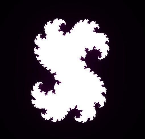
Task: Add in a mouse uniform, and normalize it in the same way the pixel position is normalized (i.e. repeat the calculation but using mouse instead of gl_FragCoord). Remember to uncheck the normalization KodeLife attempts and to invert the y-coordinate! Set c to the mouse position, toggle the code editor, and drag the mouse around. Take screenshots!

Step 3: Add in color

We have now uncovered astonishing complexity and beauty behind the simple dynamical rule z ↦ z² + c, but we can make even more beautiful graphics by adding in color.

To do this, we'll keep track of how many iterations a complex number undertakes before its length grows beyond 2. If we create a new variable representing this growth "escape" index

    int esci = 0;

and count how often iterated terms have length less than or equal to 2 inside the loop

        esci += int(length(zn) <= 2.0);

    float escp = float(esci) / float(ilimit);

We can then create a visual indicator of how quickly / slowly a complex number diverges under repeated iterations.

    gl_FragColor = float(in_R) * color1 + float(! in_R) * vec4(escp, 0, escp, 1);

Task: Visually track the rate of divergence of repeated iterations by adding color as above.

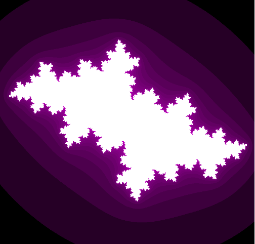
There is a slight hiccup though: many fractals do not seem to show much color. We can fix this by smoothing out the escape proportion (escp) calculation by adding logs. The difference can be dramatic, as the following two images (the first without logs, the second, with) show.

Task: Apply log() to both the numerator and denominator of the escp calculation. Discover some pretty fractals. Take screenshots! If for whatever reason you got stuck today, the final fragment shader I made is available here. (It requires uniforms to be set though.)

Bonus task: The Mandelbrot set is constructed slightly differently. If you have not made it before, look into its definition on the internet, and create it! If you have made it before, try constructing the burning ship instead.