Ithaca High School Math Seminar Lesson 2-12
Date: 2023.12.08
By the end of the previous lesson most people were able to compile Odin programs, so this morning we'll continue where lesson 2-10 ended. If you are not yet at this stage, continue following the installation instructions on the Odin website.
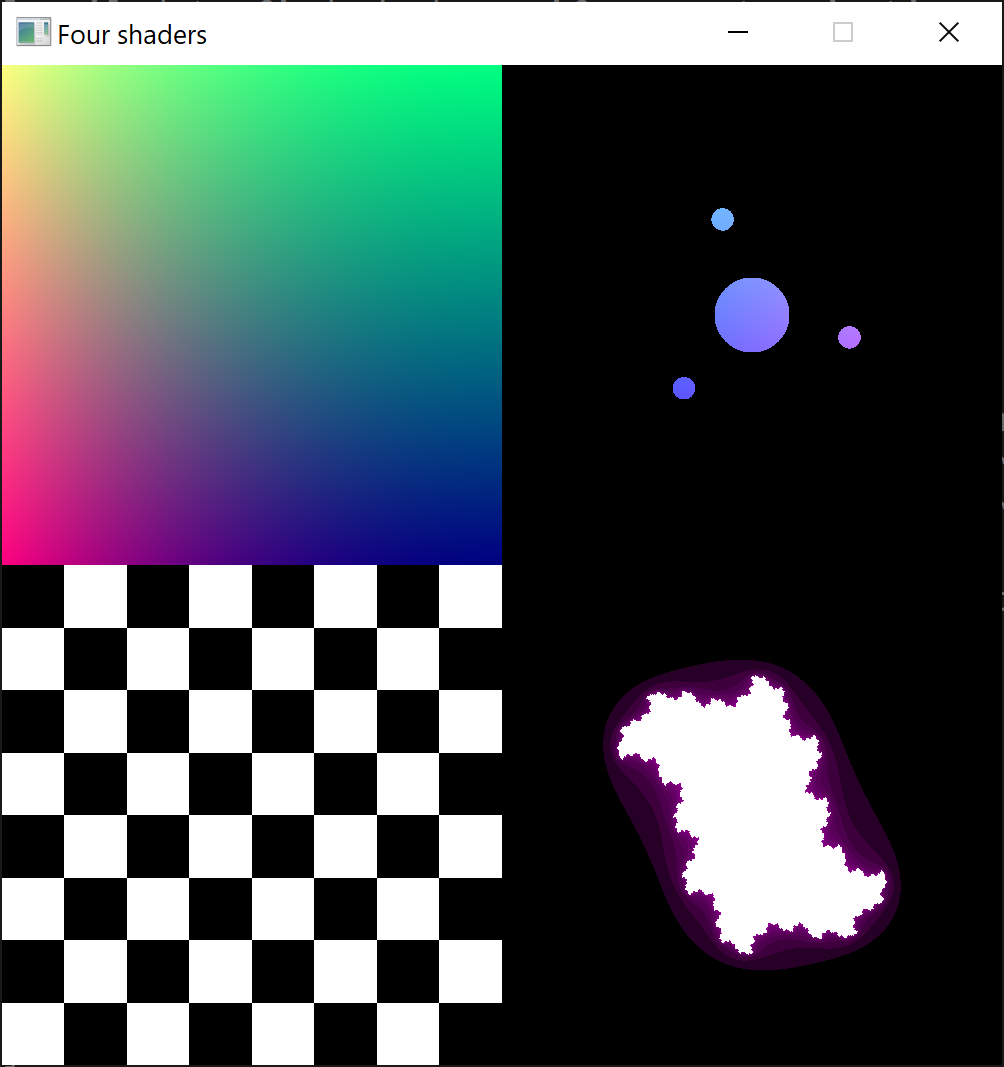
Recall that in lesson 2-10 we called some raylib procedures to draw a grid of squares with different colors. How exactly did raylib draw these? It used a shader, and since it was the default shader, we didn't need to specify it. But we can use our own fragment shaders if we want to! We'll do this today, and in the process combine them to create a showcase of the shaders we've written so far. In particular, we'll create a program that looks like the screenshot below.
Step 1: Draw a rectangle in Odin (using raylib) that displays our gradient shader
In lesson 2-3 we made a gradient shader like the following.
#version 330

// An elementary fragment shader illustrating color gradients.

void main(void)
{
    vec2 resolution = vec2(1000,1000);
    float xratio = 2 * gl_FragCoord.x / resolution.x - 1;
    float yratio = 2 * gl_FragCoord.y / resolution.y - 1;

    gl_FragColor = vec4(vec3(xratio * xratio, abs(yratio), 0.5), 1);
}
Task: Copy this shader into KodeLife to check that it works / see what it looks like. Then create a new folder, and then save the fragment shader above as a text file called color-gradient.glsl (note: Windows 11 or macOS might save the file as color-gradient.glsl.txt instead; I recommended disabling this property of Windows 11 / macOS so you know the file extensions of your files actually are. Alternatively, open up a terminal in the folder, and using the mv command change the file extension of the shader to be .glsl ).
When KodeLife visualized our fragment shader, it did so by compiling it and then running it on our GPU (which then sent the output to our screens). We can do these steps ourselves in Odin, and there are raylib procedures that help us do so quickly.
First, let's set up our project with Odin/raylib code that spaws a window with graphics.
Task: Create a new file called four-shader.odin in the folder that contains color-gradient.glsl, and fill it with the the code from lesson 2-10 that spawned a gray window. Recall that the Odin code can be compiled and run with the command odin run . called from within the folder.
Now let's fill the window with colors determined by our shader. To do so, we need to have access to our fragment shader code from within our Odin code. The easiest way to do this is to import the fragment shader as a string at compile-time using #load. I typically include this line between the first line and the start of the main procedure.
gradient_shader_code :: #load("color-gradient.glsl", cstring)
A technical note: normally we would import strings at compile-time with string instead of cstring, but since raylib is written in C, it expects strings to be stored in a different way to how Odin does by default.
Now we need to compile and load our shader. Raylib again helps us out with two procedures: LoadShader and LoadShaderFromMemory. The cheatsheet of raylib procedures on raylib's website contains a one-sentence summary of both. We loaded our shader at compile-time into gradient_shader_code, so we want to call the second raylib procedure on this.
gradient_shader := rl.LoadShaderFromMemory(nil, gradient_shader_code)
I usually include lines like these shortly after the window is initialized (i.e. after the rl.InitWindow line in the main procedure).
Now it's time to use our shader to fill in rectangles! The following lines change the shader raylib is using to our own, draws a rectangle using it, and then switches it off.
        rl.BeginShaderMode(gradient_shader)
        rl.DrawRectangle(0,0,1000,1000,rl.BLACK)
        rl.EndShaderMode()
Doing so gives us a window like the following.
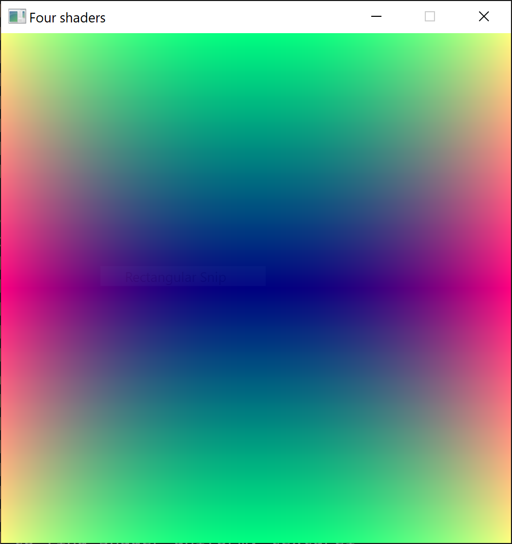
Task: Using the previous code, modify four-shader.odin to produce a window similar to the above.
Step 2: Add in the checkerboard shader
There's no reason to only use our gradient shader; we can similarly draw a rectangle filled with our checkerboard shader (checkerboard.glsl). After duplicating the steps to compile and load checkerboard.glsl that we did for the gradient shader, and modifying the sizes and locations of the rectangles, we can get a window like the following.
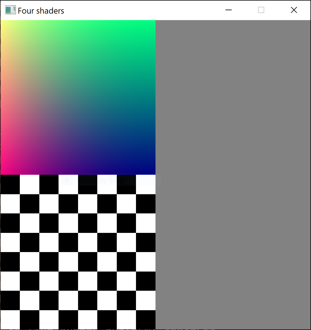
Task: After downloading the checkerboard shader (linked above) into the project, draw an additional rectangle using it to create a window like the screenshot above.
Step 3: Add in the orbiting disks shader
The shaders we've added so far have been static. Let's now add the dynamic shaders we made.
In our orbiting disk shader, the position of the orbiting disks was determined by the mouse and the time. We declared both as uniforms in our shader, and then KodeLife kept track of the time and mouse position, and updated the uniforms for us. We'll need to do both of these steps in Odin ourselves. Instead of updating both the mouse and the time, for simplicity in this lesson we'll just update the time (although the mouse is not too different), as we'll see later.
Let's add a stopwatch to our main procedure, and start it before we launch any window.
    // Start a clock.
    watch : time.Stopwatch
    time.stopwatch_start(&watch)
    // The variable we'll set the uniform time to.
    seconds : f32
These stopwatch structs and procedures are part of Odin's core time library, which we can use after we import it.
import "core:time"
Now we have a stopwatch in Odin, but to pass in a time value to our shaders, we'll need to read the stopwatch, and convert its time into seconds. Let's do this at the start of every rl.WindowShouldClose() loop.
        raw_duration := time.stopwatch_duration(watch)
        seconds = f32(time.duration_seconds(raw_duration))
Now we have a variable (seconds) whose value every frame is the time since the program began running. Let's use it in our orbiting disks shader (disks.glsl).
Assume that we imported, compiled, and loaded the code of disks.glsl with
    disks_shader_code :: #load("disks.glsl", cstring)
    disks_shader := rl.LoadShaderFromMemory(nil, disks_shader_code)
The location of the time uniform in our shader is somewhere in memory, and before we update it, we need to determine where it is. We can use the following raylib procedure to do this before we initialize the window.
disks_time_loc := rl.GetShaderLocation(disks_shader, "time")
Now with the location of the time float in our shader, we can update it with our stopwatch time. In the main loop body, but before we start drawing, let's set the time uniform.
    // Set time uniforms.
    rl.SetShaderValue(disks_shader,
                      cast(rl.ShaderLocationIndex) disks_time_loc,
                      &seconds,
                      .FLOAT)
We can now use our shader to render geometry in our program.
        rl.BeginShaderMode(disks_shader)
        rl.DrawRectangle(500,0,500,500,rl.BLACK)
        rl.EndShaderMode()
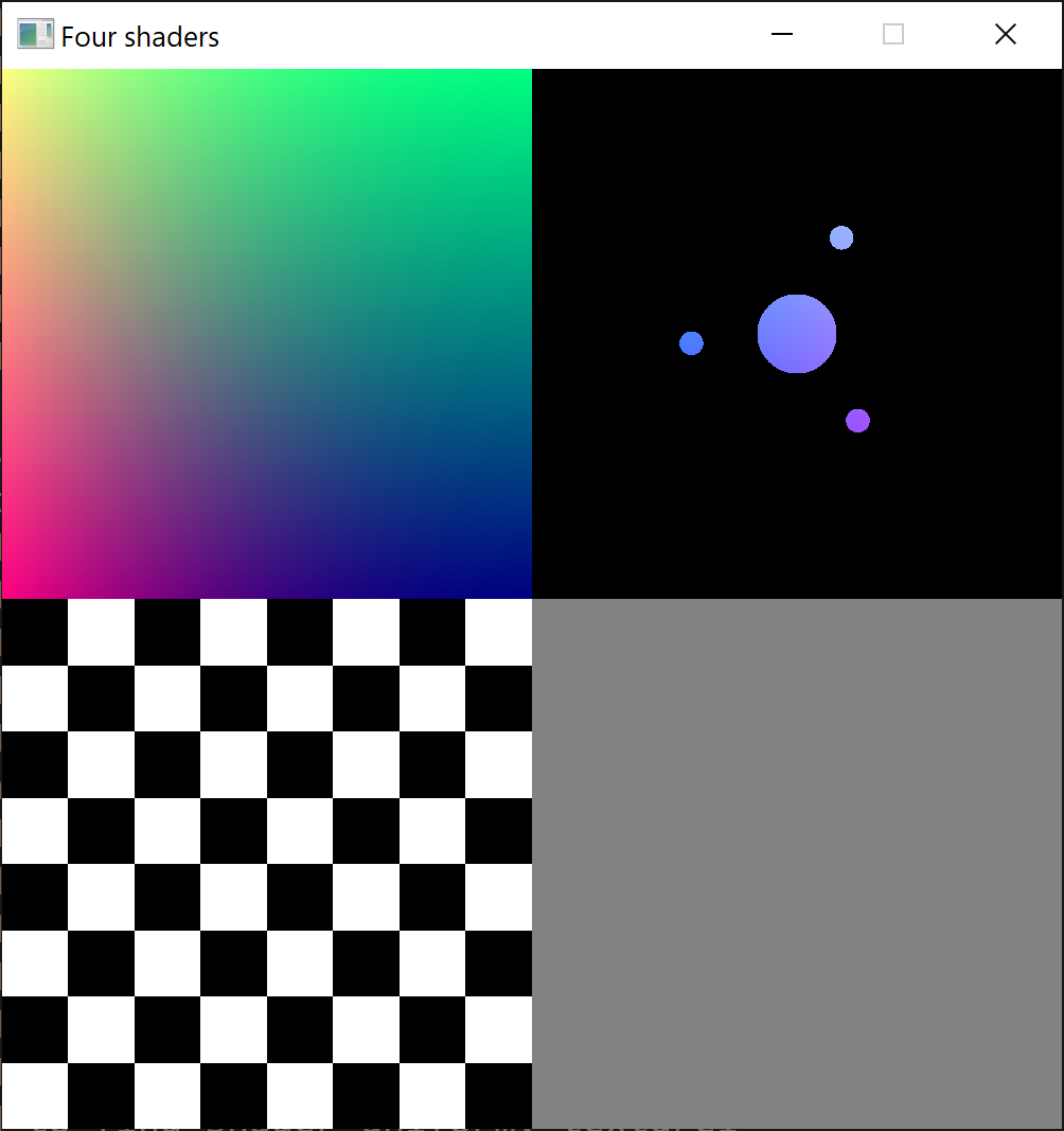
Task: As above, include the orbiting disk fragment shader (linked above) into the project, add in a stopwatch to the program, and use it to update the shader to make the image it draws dynamic. Note: for simplicity, by default the disk shader draws the disks in the top-right corner by manually setting the mouse uniform to this position.
Step 4: Add in the Julia set shader
Similar to above, it's also possible to pass in the mouse position to our shaders, but again for simplicity we'll just stick with the time today. I've modified the Julia set shader so that the c value in the iteration is determined by time instead of the mouse position, and drawn in the bottom-right corner. The modified version is here: (julia-sets.glsl).
Final Task: Incorporate the Julia set shader into the program to make something like the image at the top of this page. Since the program already has a stopwatch, there is no need to create a second stopwatch, however, like the orbiting disks shader, the location of the time uniform in the for the Julia set shader will need to be located and updated.
If you've got this far: congratulations! In less than 10 hours, we've made four very different shaders from scratch, and created our own program that visualizes them. Imagine what we could do with even more time.
We've covered a lot, but our graphics have all been 2-dimensional. A lot of computer graphics are 3-dimensional; how could we go about making these?
Doing so involves a lot of work, and looking into this in detail would certainly take more time than the four lessons remaining. But we can try to at least glimpse some of the ideas involved! In the process, we'll see how linear algebra is fundamental to the creation of 3-dimensional graphics.